Geophysical Exploration of Crustal Structure

Exercise 6: Supplement

Deconvolution

Following is an example of this instruction. Note that there is no "sample.su" provided.

Display the autocorrelation of "sample.su".

$ suacor < sample.su sym=0 | suxwigb &

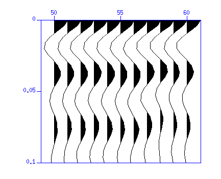
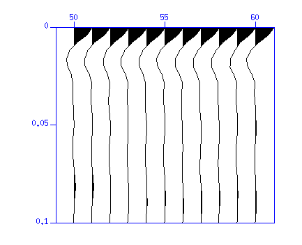
The autocorrelation indicates the repetition of about 0.04s second is dominant. Therefore, to remove the autocorrelation after the second peak, apply a prediction-error-filter (deconvolution) whose prediction length is 0.03 seconds. The autocorrelation after deconvolution shows that the repetitions are removed.

$ supef minlag=0.03 < sample.su | suacor sym=0 | suxwigb &

Fig: (A portion of) autocorrelation. (Left) Original. The repetition of about 0.04 seconds is dominant. (Right) After deconvolution. The repetitions are removed.

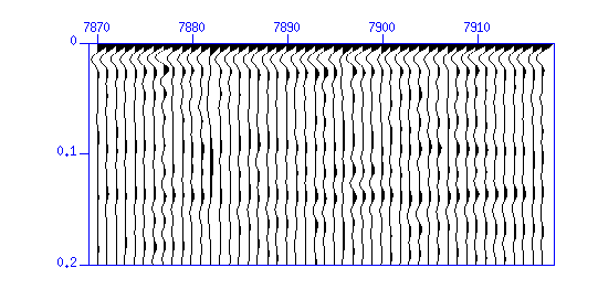
Display the autocorrelation of "cdp_1095_flt_gain.su".

$ suacor < cdp_1095_flt_gain.su sym=0 | suxwigb &

Referring the autocorrelation, apply deconvolution using an appropriate value for 'minlag'. You will need some trial-and-errors to find an appropriate value by referring waveforms and autocorrelations.

$ supef minlag=???? < cdp_1095_flt_gain.su | suxwigb &
$ supef minlag=???? < cdp_1095_flt_gain.su | suacor sym=0 | suxwigb &

$ supef minlag=???? < cdp_1095_flt_gain.su | sufilter f=?,?,?,? amps=0,1,1,0 > cdp_1095_flt_gain_decon.su