waterPMLコマンドの検証

6. ランダムに配置した力源を用いた計算

(Examples and validations for waterPML command — 6. computation using randomly distributed sources)

◆概要と問題設定 (Outline and the problem)

雑微動を用いた地震波干渉法は地下構造推定のために広く用いられている。数値シミュレーションを用いた地震波干渉法の理論的研究のために waterPMLコマンドを用いることができる。その手順を示すための、ごく単純化した例題である。
Seismic interferometry of ambient noise is widely used to investigate subsurface structures. The waterPML command is applicable to a numerical simulation-based theoretical study of the seismic interferometry. A simplified example to show the procedure of the numerical simulation is described below.

数値シミュレーションの流れは以下の通りである。観測網を囲むようにランダムに力源を配置し、各観測点での理論波形をwaterPMLコマンドを用いて計算する。次に、観測点間の波形の相互相関関数を計算し、それを用いて地下構造を求め、理論波形計算に用いた地下構造(正解)に近いものが得られるかを検証する。この一連の流れの中でwaterPMLコマンドを用いるのは理論波形計算の部分であるので以下ではその手順を説明する。簡単のため、この例題では観測点を2つのみ用いる(観測点数が増えても処理の流れは変わらない)。使用するレイアウトを図1に示す。
A study flow of the numerical simulation is as follows. Deploy seismic wave sources randomly that surround a station network, and compute theoretical waveforms at individual stations using waterPML command. Next, compute the cross correlation function (CCF) between each pair of stations, investigate the subsurface structure from the CCFs, and compare the estimated subsurface structure with the true one that was used to compute the theoretical waveforms. The description below focuses on the computation of theoretical waveforms, where waterPML command is used. For simplicity, only two stations are used in this example; increasing the number of stations does not change the procedures. Fig. 1 shows the configuration used.

図1. 問題設定。(a)水平面、(b)$y=0$の鉛直断面。地形を(a)に色と等値線(100 m間隔)で、(b)に茶色で示す。 (b)の薄い茶色は低速度の表層、濃い茶色は高速度の半無限媒質を表す。 ★は地震波動ソースの位置、 ▲は観測点の位置を表す。
Fig. 1. The problem to be solved in (a) horizontal section and (b) a vertical section along $y=0$. The light and dark browns in (b) represent a low-velocity surface layer and a high-velocity half space, respectively. The topography is shown by color scale and contours (100 m intervals) in Fig. 1a and brown in Fig. 1b. The star (★) and triangles (▲) indicate the locations of the seismic wave source and stations, respectively.

以下、理論波形計算で使用するパラメータとその決定方法(考え方)を説明する。
The description below focuses on how to determine the parameters used to compute theoretical waveforms.

●地震波速度構造 (The velocity structure)

使用する地震波速度構造を最初に決めるのが良い。それに応じて適切な格子セルのサイズや物理領域の大きさ等が変わってくるからである。
It is recommended to determine the velocity structure first, because it affects the appropriate grid cell size and the width of the physical volume.

この例題では簡単のため、 P波速度$V_p=5000$ m/sの半無限媒質の上に $V_p=3000$ m/sの表層(厚さ1000 m)が乗った2層構造を考える。 S波速度$V_s=V_p/\sqrt{3}$、密度$\rho$ [kg/m$^3$]$=1740V_p$[km/s]$^{0.25}$ (Gardner et al. 1974) とする。
For simplicity, a two-layer structure is considered in this example, composed of a half-space with a P-wave velocity $V_p=5000$ m/s overlain by a surface layer with $V_p=3000$ m/s and a thickness of 1000 m. For each layer, an S-wave velocity $V_s=V_p/\sqrt{3}$ and a density $\rho$ [kg/m$^3$]$=1740V_p$[km/s]$^{0.25}$ (Gardner et al. 1974) are used.

この速度構造を与える地下構造の設定ファイルの例を以下に示す。物理領域の空間範囲は後で考えるが、地下構造の定義域が物理領域よりも広い分には構わないのでここでは余裕を持たせて海抜下20 kmまでの地下構造を定義している。
An example of a structure file for this subsurface structure is shown below. The spatial range of the physical volume is considered later; however, the definition range of the subsurface structure can be wider than that of the physical volume. Therefore, the subsurface structure is defined down to 20 km below sea level to make sure that the definition range is wider than the physical volume.

(structure6.ini)

surface+0.1[TAB]3000.0[TAB]1732.1[TAB]2290.0
surface-999.9[TAB]3000.0[TAB]1732.1[TAB]2290.0
surface-1000.1[TAB]5000.0[TAB]2886.8[TAB]2601.9
-20000.1[TAB]5000.0[TAB]2886.8[TAB]2601.9

地震波干渉法で主に用いられるのはレイリー波である。その伝播速度は周波数によって異なる。低周波では深部の地震波速度が反映されるため高速度になり、高周波では浅部の地震波速度が反映されるため低速度になる。最も遅い波は高周波極限でのレイリー波であり、これは表層の速度である$V_p=3000$ m/sの均質媒質中のレイリー波の速度を考えれば良いのでおおよそ$0.9V_s\sim 1500$ m/s程度である。一方、計算する波動場に含まれる最も速い波は半無限媒質中のP波(5000 m/s)である。したがって、この例題では1500-5000 m/sの波が波動場に含まれる想定で計算のパラメータを設定すれば良い。
Seismic interferometry mainly uses Rayleigh wave, whose velocity depends on frequency; the velocity is relatively fast (slow) in low (high) frequency because it is determined by the velocity in deep (shallow) parts. The slowest wave is Rayleigh wave in high-frequency limit, whose velocity is approximated by a Rayleigh wave velocity in a homogeneous medium with $V_p=3000$ m/s (the velocity of the surface layers), i.e., $0.9V_s\sim 1500$ m/s. The fastest wave in the simulated wave field is the P-wave in a half space (5000 m/s). Therefore, parameters for this example should be determined assuming wave propagation velocities between 1500 and 5000 m/s.

●震源時間関数と格子セルのサイズ (Source time function and grid cell size)

地震波干渉法では海洋波浪による脈動が波動源として想定される場合が多い。この例題でもこれを念頭に置き、 0.5 Hzのローパスフィルターを掛けた乱数時系列データを震源時間関数として用いることにする。
Seismic interferometry usually assumes a microseismic noise caused by ocean wave as the noise source. Following it, this example uses a random time series data low-pass filtered at 0.5 Hz for the source time function.

この場合、波動に含まれる最小の振動周期は約2 sであるので、上で考えた1500-5000 m/sの伝播速度を用いると最小の波長は約3000 mになると予想される。このことを踏まえて格子セルのサイズは100 mとする。この場合、1波長あたり30格子セル以上を確保できる。
This means that the minimum oscillation period of the wave contained in the simulated wave field is ~ 2 s, which corresponds to a minimum wave length of ~ 3000 m according to the wave propagation velocity of 1500-5000 m/s considered above. Based on this estimation, we use a grid cell size of 100 m, which realizes $\geq 30$ grid cells in a wave length.

●観測点 (Stations)

地震波干渉法が成功すると相互相関関数の波形において 2観測点間の走時に対応する時間差のところにパルスが出現する。観測点間距離が短い場合、このパルスが時間差0をまたいでしまい、成否の判断が難しくなる。そこで、パルスが時間差0から十分離れた時刻に出現するには観測点間をどの程度離せば良いかを考えて観測点配置を決定する。今回の例題では波動場に含まれる最も短い周期が2 s、最も速い速度が5000 m/sであった。そこで、パルスが時間差2 sよりも後に出現するように観測点間を10000 m離せば、得られた波形にハイパスフィルターを掛けて周期2 sの振動成分を取り出したときに地震波干渉法の成否を判断できると期待される。このことを踏まえて、今回の例題では2つの観測点の水平位置を $(5000,0)$および$(-5000,0)$ (単位:m)とする。下記が観測点のリストファイルである。
If seismic interferometry successes, the resultant CCF has a pulse at the lag time corresponding to the travel time between the two stations. If the distance of the two stations is too short, this pulse lies over the zero lag time, which makes it difficult to identify the success of the seismic interferometry. To avoid this scenario, consider the minimum station distance that would realize the pulse at a lag time that is sufficiently apart from the zero lag time. The minimum oscillation period of 2 s in the simulated wave field and the fastest propagation velocity of 5000 m/s in the present example suggests that the pulse would be located at a lag time larger than 2 s if the stations are 10000 m apart; in this case, the success of the seismic interferometry could be examined by applying a high-pass filter to simulated waveforms to extract an oscillation of 2-s period. Therefore, this example uses stations located at $(5000,0)$ and $(-5000,0)$ (unit: m). The corresponding station list file is shown below.

(station_list6.dat)

STN1[TAB]5000.0[TAB]0.0[TAB]surface-0.1
STN2[TAB]-5000.0[TAB]0.0[TAB]surface-0.1

●力源 (Seismic wave sources)

この例題では観測点を囲む円環状の領域において、地表直下の格子セルに鉛直シングルフォースの力源を与える。最も短い3000 mの波長において力源から観測点まで1波長以上の距離を確保するため、 (0,0)を中心とする半径8000-9000 mの円環領域に力源を配置する。その面積は$5.3\times 10^7$ m$^2$であるので 100 m$\times$ 100 mの格子セルが約5300個入ることになる。その1/10に当たる500個の力源を円環領域内にランダムに配置する。このとき力源は円環領域を埋め尽くすのではなく円環領域内に疎にランダムに配置されることになる。
In this example, vertical single forces are placed at grid cells immediately beneath the ground surface in a doughnut-shaped region that surrounds the stations. The doughnut has a radius of 8000-9000 m and is centered on (0,0) to keep a distance from stations greater than or equal to the smallest wave length of 3000 m. The area of the doughnut is $5.3\times 10^7$ m$^2$, which includes ~ 5300 grid cells of 100 m$\times$ 100 m size. A total of 500 source forces, which is approximately 1/10 of the number of grid cells, are distributed randomly in this area. Therefore, the source forces are relatively sparce rather than filling out the doughnut.

ランダムに分布する力源の設定ファイルは create_tws_source_config_randomコマンドを用いると簡単に作成できる。今回の例題の条件に合わせた設定ファイルを作成するコマンドを以下に示す。
A configuration file for the randomly distributed seismic wave sources can be created easily by create_tws_source_config_random command. The command for the present example is shown below.

create_tws_source_config_random --output_config_file=source6.ini --output_coordinate_list_file=source_coordinate6.dat --geometry=surface_circle --x0=0.0,0.0 --r_min=8000.0 --r_max=9000.0 --d_min=0.1 --d_max=99.9 --number=500 --dx_min=100.0 --mechanism=Fz --stfun_tp=2.0 --stfun_ts=2.0

●地形データ (Topography data)

waterPMLコマンドの特色の1つは3次元地形を計算に入れられることである。この例題においても3次元地形を用いて計算を行う。ここでは例として、ガウス関数 \[\begin{equation} h(x,y)=h_0+\Delta h \exp\left(-\frac{x^2+y^2}{r^2}\right) \label{eq.topography} \end{equation}\] で表される地形を使用する。ここで$h_0$は無限遠方での地表面の標高、 $\Delta h$は中心部での地形の盛り上がり(山体)の比高、 $r$は地形の盛り上がりの水平方向の距離スケールである。
An advantage of waterPML command is that it can incorporate 3-D topography into the computation. This example uses a Gaussian function (Eq. \ref{eq.topography}) as a 3-D topography, where $h_0$ is the ground surface evelation at an infinite distance, $\Delta h$ is the relative height of mountain at the center, and $r$ is the horizontal distance scale of the mountain.

(\ref{eq.topography})式のパラメータは表1のように設定する。
Parameters in Eq. (\ref{eq.topography}) are listed in Table 1.

表1. (\ref{eq.topography})式のパラメータ。
Table 1. Parameters in Eq. (\ref{eq.topography}).

パラメータ Parameter	値 Value
$h_0$	500 m
$\Delta h$	1500 m
$r$	5000 m

この地形データを作成するコマンドを以下に示す。ここでは後述の物理領域をカバーするように地形データの定義域を$-10100 \leq x,y\leq 10100$ (単位:m)とした。
A command to create this topography data is shown below. Here, the definition range of the topography data of $-10100 \leq x,y\leq 10100$ (unit: m) was selected to include the physical volume described later.

rm -f topography_ex6.dat
for((x=-10100;x<=10100;x+=100))
do
  for((y=-10100;y<=10100;y+=100))
  do
    echo $x $y | awk '{ h0=500.0; delta_h=1500.0; r=5000.0; h=h0; distance2=$1*$1+$2*$2; if(distance2<100.0*r*r){ h=h0+delta_h*exp(-distance2/(r*r)); } printf("%d\t%d\t%f\n",$1,$2,h); }' >> topography_ex6.dat
  done
done

ここでは警告を避けるため、expの中身が-100よりも大きい場合のみ各項を加算するように場合分けした。
Here, each term is added only if the content of exp is greater than -100 to avoid warning.

●物理領域 (Physical volume)

地震波動ソースを置く場所から物理領域の端までの間に10格子セル以上を確保し、かつ(0,0)が格子セルの中心点になるようにするため、物理領域の水平座標範囲を$-10050\leq x,y\leq 10050$ (単位:m)とする。
The horizontal coordinate range of the physical volume is set as $-10050\leq x,y\leq 10050$ (unit: m) to keep $\geq$ 10 grid cells from source locations to the nearest boundary of the physical volume and to make (0,0) at the center of a grid cell.

表1より地表面の標高が最も高い場所で2000 mであるので、その上に真空の格子セルを2つ設けて物理領域の上端を標高2200 mとする。レイリー波を適切に表現するため、地表面(最小:標高500 m; 表1)から物理領域の下端までに最小の波長の2波長分にあたる6000 mの厚みを確保する。これにより、物理領域の標高の下端は-5500 mとなる。
The upper bound of the physical volume is set at 2200 m above sea level to realize two vacuum cells above the summit of the ground surface at 2200 m above sea level. To properly express a Rayleigh wave, a thickness of 6000 m (three times the minimum wave length) is preserved between the ground surface (lowest: 500 m above sea level; Table 1) and the bottom of the physical volume; therefore, the lower bound of the physical volume is -5500 m.

物理領域の範囲をこのように設定した場合、格子セル数は$201\times 201\times 77$となる。これまでの例題よりも格子セルの個数は多いが、この個数であればメモリの使用量は6GB程度であるのでそれほど高価でないコンピュータを用いて計算可能である。
This physical volume has $201\times 201\times 77$ grid cells. This number is larger than those in previous examples, but small enough to consume only ~ 6 GB memory, so the computation is possible with a computer that is not so expensive.

●問題設定のプロット (Plotting the problem setting)

waterPMLコマンドを実行する上で必須ではないが、 Generic Mapping Tools (version 6) を用いて図1をプロットするコマンドを以下に示す。
Although it is not required for running waterPML, commands to generate Fig. 1 by Generic Mapping Tools (version 6) are shown below.

gmt begin problem6 ps

gmt set FONT_ANNOT_PRIMARY 12p

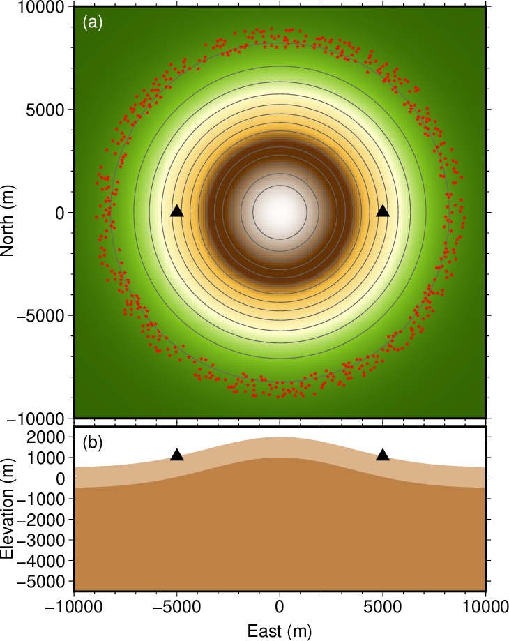
#地形のプロット(水平面)
#Plotting topography in horizontal section
gmt surface topography_ex6.dat -R-10000/10000/-10000/10000 -I100/100 -Gtopography_ex6.grd

gmt makecpt -Cdem1 -T500/2000/10 -Z -D

gmt grdimage topography_ex6.grd -R-10000/10000/-10000/10000 -JX10/10 -Xa3 -Ya7.2

gmt grdcontour topography_ex6.grd -R-10000/10000/-10000/10000 -JX10/10 -Xa3 -Ya7.2 -C100 -W0.4,100/100/100 -Bxa5000f1000 -Bya5000f1000 -BWsen

#表層のプロット(東西断面)
#Plotting the surface layer in EW section
awk '($2==0){ print $1,$3 } END{ printf("10000\t-5500\n"); printf("-10000\t-5500\n"); }' topography_ex6.dat | gmt plot -R-10000/10000/-5500/2500 -JX10/4 -Xa3 -Ya3 -G220/180/140

#半無限媒質のプロット(東西断面)
#Plotting the half space in EW section
awk '($2==0){ print $1,$3-1000.0 } END{ printf("10000\t-5500\n"); printf("-10000\t-5500\n"); }' topography_ex6.dat | gmt plot -R-10000/10000/-5500/2500 -JX10/4 -Xa3 -Ya3 -G190/130/70 -Bxa5000f1000 -Bya1000 -BWSen

#地震波動ソースのプロット
#Plotting seismic wave sources
awk '{ print $2,$3 }' source_coordinate6.dat | gmt plot -R-10000/10000/-10000/10000 -JX10/10 -Xa3 -Ya7.2 -Sa0.1 -G255/0/0

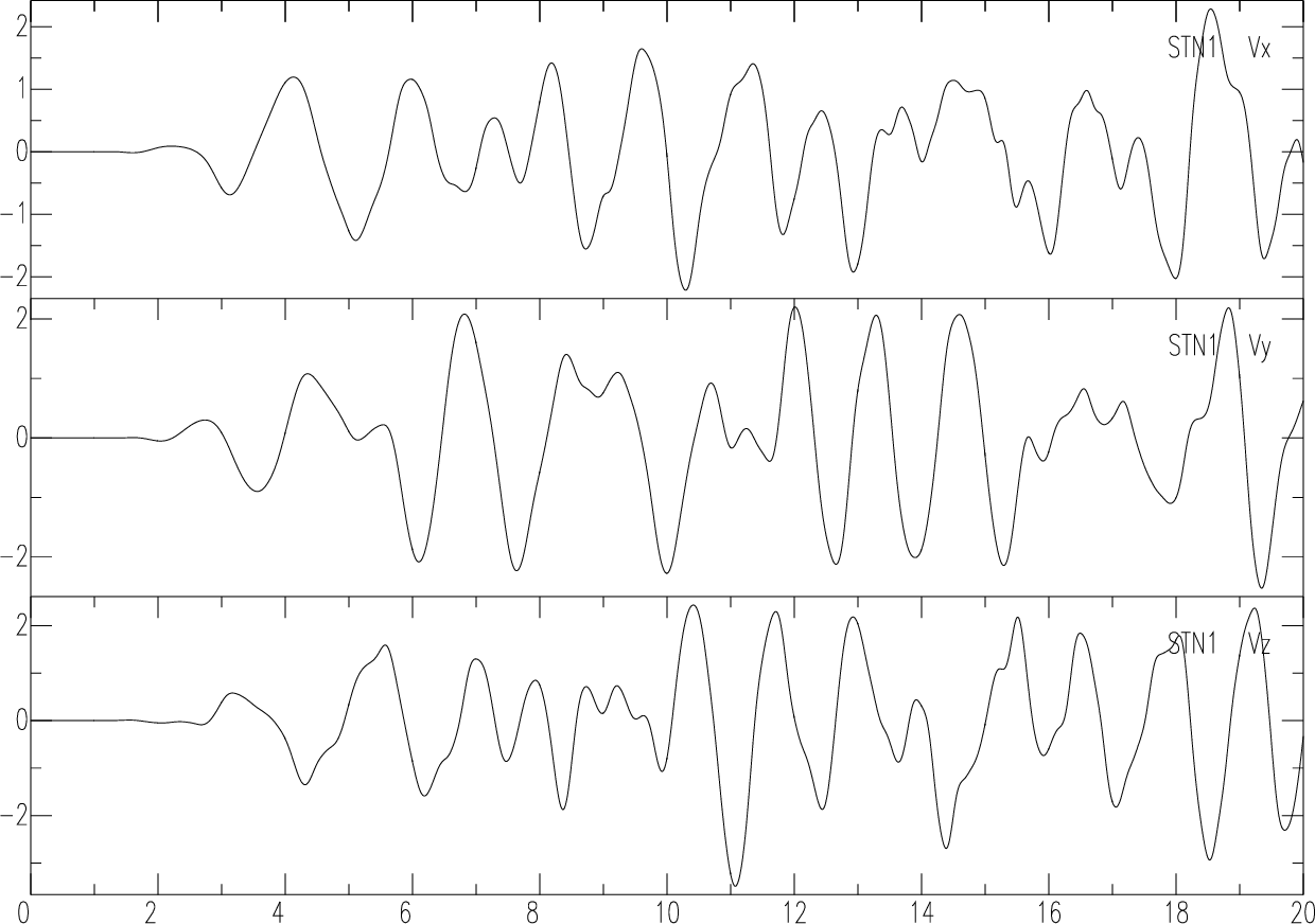
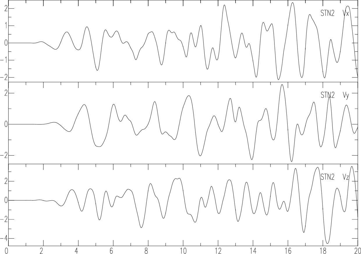
#観測点のプロット
#Plotting stations
gmt plot -R-10000/10000/-10000/10000 -JX10/10 -Xa3 -Ya7.2 -St0.4 -G0/0/0 <<EOF
-5000 0
5000 0
EOF

station_z=`awk '($1==5000 && $2==0){ print $3 }' topography_ex6.dat`
gmt plot -R-10000/10000/-5500/2500 -JX10/4 -Xa3 -Ya3 -St0.4 -G0/0/0 <<EOF
-5000 $station_z
5000 $station_z
EOF

#文字列のプロット
#Plotting texts
gmt text -R0/21/0/29.7 -JX21/29.7 -Xa0 -Ya0 -F+f12p+a+j <<EOF
8.0 2.2 0 CT East (m)
1.5 12.0 90 CB North (m)
1.5 5.0 90 CB Elevation (m)
3.2 6.8 0 LT (b)
EOF

gmt text -R0/21/0/29.7 -JX21/29.7 -Xa0 -Ya0 -F+f12p,,255/255/255+a+j <<EOF
3.2 17.0 0 LT (a)
EOF

gmt end

◆計算 (The calculation)

計算には以下のコマンドを用いる。
Use the command below to perform the calculation.

waterPML --Nx=201 --Ny=201 --Nz=77 --Npmx=20 --x0=-10050.0 --y0=-10050.0 --z0=-5500.0 --dx=100.0 --dt=0.01 --tmax=20.0 --topography_files=topography_ex6.dat --topography_file_format=xy --structure_file=structure6.ini --structure_file_format=layer --source_file=source6.ini --source_memory=smaller --output_dir=result06 --station_file=station_list6.dat

これまでの例題との大きな違いは赤字で示した --source_memory=smallerオプションである。これはymaeda_opentools version 2025-01-21aで導入した機能である。従来は物理領域内の位置と等価体積力の配列要素番号との関係を全ての格子セルの中心や境界について記憶していた。力源が1つや2つであればこのことが大きな問題になることは無かったが、この例題のように500個の力源を用いる場合、従来方式ではコンピュータメモリが不足する。 --source_memory=smallerオプションを用いると新方式のコードが用いられ、この中では物理領域内の位置と等価体積力の配列要素番号との関係を等価体積力が必要な場所についてのみ記憶する。そのため等価体積力に使用するコンピュータメモリを抑制でき、 500個のような多数の力源を与えた計算が可能になる。
The main difference between this and previous examples is the use of --source_memory=smaller option shown by red, which was introduced in ymaeda_opentools version 2025-01-21a. The conventional computation code remembered the relation between every location (at the centers or boundaries of grid cells) in the physical volume and the corresponding array index for an equivalent body force. This was not a serious problem as long as only one or two seismic wave sources were used; however, this results in a huge computer memory requirement when as many as 500 seismic wave sources are used, which is the case of this example. The --source_memory=smaller option results in the use of a revised computation code, which remembers the relation between only the locations in the physical volume where an equivalent body force is needed and the corresponding array indices for the equivalent body force, thereby suppressing the memory requirement for equivalent body force and realizing the computation with a lot of (e.g., 500) seismic wave sources.

◆事後処理 (Postprocessings)

●計算結果の確認 (Checking the results)

計算した波形はresult06/waveformディレクトリの下に格納される。観測点STN1の速度波形はSTN1.Vx.seq1, STN1.Vy.seq1, STN1.Vz.seq1であり、観測点STN2の速度波形はSTN2.Vx.seq1, STN2.Vy.seq1, STN2.Vz.seq1である。
The waveforms computed by the command above are stored under result06/waveform directory; STN1.Vx.seq1, STN1.Vy.seq1, and STN1.Vz.seq1 are the velocity waveforms at station STN1, and STN2.Vx.seq1, STN2.Vy.seq1, and STN2.Vz.seq1 are those at station STN2.

波形を確認するには sequence2sac_timeseqコマンドを用いてSeismic Analysis Code (SAC)の時系列データに変換し、 SACソフトウェアを用いてプロットするのが簡単である。
An easy way to check the waveforms is to convert into time series data of Seismic Analysis Code (SAC) format using sequence2sac_timeseq command, and then plot them using SAC software.

ところで今回計算した速度波形の最大振幅は$10^{-14}$ m/sの桁になっている。これは力源の強度を指定しておらず、デフォルトの1 Nが用いられたためである。このような小さな振幅の波形は後に相互相関関数を計算する際に不都合がある (ymaeda_opentoolsではあまりにも小さい実数は0と見なす仕組みを用いているため、および相互相関関数の計算式の分母が波形の振幅の2乗に比例するため)。そこで、SAC形式に変換後、波形全体に$10^{14}$を掛けることにより、 $10^0$の桁になるように規格化しておくのが良い。
The maximum amplitudes of the velocity waveforms are order of $10^{-14}$ m/s. These small amplitudes were caused by omitting the source intensity; a default source intensity of 1 N was used. Waveforms with the small amplitudes would cause a problem in calculation of CCFs (performed later) because ymaeda_opentools regards extremely small real numbers to be zero, and the denominator of CCFs is proportional to the square of wave amplitudes. To avoid this problem, multiply $10^{14}$ to the entire waveforms after the conversion to the SAC format to normalize the amplitude levels to order of $10^0$.

SAC形式への変換、$10^{14}$倍、波形のプロットを行うコマンドを以下に示す。
The commands below consist of conversion to SAC format, multiplying $10^{14}$, and plotting the waveforms.

cd result06/waveform

for file in *.seq1
do
  file=`basename $file .seq1`
  sequence2sac_timeseq $file.seq1 $file.sac
  sac <<EOF
  r $file.sac
  mul 1.0e+14
  w $file.sac
  q
EOF
done

sac <<EOF
bd sgf
qdp off
r STN1.Vx.sac STN1.Vy.sac STN1.Vz.sac
ch KSTNM STN1
ch file 1 KCMPNM Vx
ch file 2 KCMPNM Vy
ch file 3 KCMPNM Vz
p1
r STN2.Vx.sac STN2.Vy.sac STN2.Vz.sac
ch KSTNM STN2
ch file 1 KCMPNM Vx
ch file 2 KCMPNM Vy
ch file 3 KCMPNM Vz
p1
q
EOF

sgftops f001.sgf STN1.ps
sgftops f002.sgf STN2.ps
rm -f *.sgf

プロットした波形を図2,図3に示す。高周波の振動は抑制されており、低周波の振動はランダムであることからおおよそ意図通りの計算ができたと思われる。
Figs. 2 and 3 show the waveforms plotted in this way. High-frequency oscillations are suppressed, and low-frequency oscillations show randomness, suggesting that the computation basically succeeded.

図2. 観測点STN1の速度波形。
Fig. 2. The velocity waveforms of station STN1.

図3. 観測点STN2の速度波形。
Fig. 3. The velocity waveforms of station STN2.

●相互相関関数の計算 (Computation of CCFs)

相互相関関数は sacfile_correlationコマンドを用いて計算できる。ここでは例として観測点STN1とSTN2の上下成分同士の相互相関関数を計算・プロットするコマンドを示す。
The CCFs can be computed using sacfile_correlation command. Here, commands to compute and plot the CCF between the vertical component at stations STN1 and STN2 are shown as an example.

sacfile_correlation STN1.Vz.sac STN2.Vz.sac correlation.zz.sac

sac <<EOF
bd sgf
qdp off
r correlation.zz.sac
p1
q
EOF

sgftops f001.sgf correlation.zz.ps
rm -f *.sgf

プロットした相互相関関数の波形を図4に示す。ラグタイム$\pm 5$ s付近を先頭にシグナルが到着していることが分かる。今回の例題では観測点間距離は10 kmであった。第1層のP波速度が3 km/sであるので、浅部の地震波速度が反映される高周波極限でのレイリー波速度は $0.9V_s\sim 1.5$ km/sであり、仮にこの速度で観測点間を波が伝播した場合には走時6-7 s程度になる。また第2層(半無限媒質)のP波速度が5 km/sであるので、深部の地震波速度が反映される低周波極限でのレイリー波速度は $0.9V_s\sim 2.6$ km/sであり、仮にこの速度で観測点間を波が伝播した場合には走時4 s程度になる。その中間にあたる5 s程度の走時で波群が到達していることから地震波干渉法のシミュレーションとしては成功と見なしうるものである。 0 s付近にも強いシグナルが残っているのは地震波動ソースの個数が500個と比較的少ないこと、地震波動ソースから観測点までの距離が最短3 km(最小波長の1波長分)と短いこと、地表から物理領域下端までの厚みが6 km(最小波長の2波長分)程度しか無いために特に低周波成分はレイリー波が十分に減衰する深さまで計算できていない可能性があること、計算した波形の長さも20 sと比較的短いことが原因として考えられる。これらの問題を解決してより精度の高い計算を行うにはより多くのメモリと計算時間を使う計算が必要になる。
Fig. 4 shows the waveform of the CCF, which consists of signals that arrive at $\pm 5$ s. Given an inter-station distance of 10 km and a P-wave velocity of the 1st layer of 3 km/s, the Rayleigh wave velocity in the high-frequency limit is $0.9V_s\sim 1.5$ km/s and the corresponding travel time is 6-7 s; and given a P-wave velocity of the 2nd layer (half space) of 5 km/s, the Rayleigh wave velocity in the low-frequency limit is $0.9V_s\sim 2.6$ km/s and the corresponding travel time is approximately 4 s. Therefore, the observed arrival time of 5 s in Fig. 4 is in the possible range of theoretical travel times of the Rayleigh wave, suggesting some success of seismic interferometry. Another strong signal near 0 s lag time suggests insufficient accuracy of computation caused by, e.g., a relatively small number (500) of seismic wave sources, a relatively short distance (3 km; comparable to the smallest wave length) from seismic wave sources to stations, a relatively small thickness (6 km; comparable to twice the smallest wave length) from the ground surface to the bottom of the physical volume that may not be able to properly express the reduction of Rayleigh wave amplitudes along the depth especially in low frequency, and a relatively short length (20 s) of the waveforms computed. Higher computation accuracy may be achieved by resolving these problems which, however, requires additional computational memory and time.

図4. 観測点STN1とSTN2の上下成分同士の相互相関関数。
Fig. 4. Cross correlation function between the vertical component of stations STN1 and STN2.

パラメータ Parameter	値 Value
\(h_0\)	500 m
\(\Delta h\)	1500 m
\(r\)	5000 m