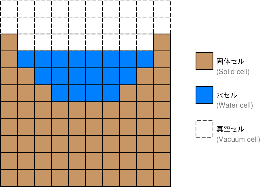
図1. waterPMLコマンドにおける地形と水域の表現方法の模式図。
Fig. 1. Schematic illustration for the representations of the topography and water-filled regions in waterPML command.
|
図1. waterPMLコマンドにおける地形と水域の表現方法の模式図。 Fig. 1. Schematic illustration for the representations of the topography and water-filled regions in waterPML command. |
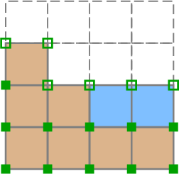 図2. 応力の非対角成分を計算する地点 (▪)、 計算をスキップして初期値(0)のままにする地点 (▫)。 Fig. 2. Locations where the off-diagonal stress components are computed (▪) and where the computation is skipped to keep them at their initial values of zero (▫). |
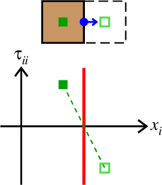 図3. 地表面(や水面)で法線応力を0にするための考え方。 ▪ が計算に登場する固体セル内の法線応力、 ▫ が仮想的に考える真空中の法線応力であり、 後者が前者の\(-1\)倍であるものとして 境界面での速度の法線成分(青)を計算する。 Fig. 3. A schematic illustration for the free surface boundary condition for a normal stress component on a ground (or water) surface. An imaginary normal stress in the vacuum (▫) is assumed to be \(-1\) times that in the solid cell (▪) in the computation of the normal velocity component on the boundary (blue). |
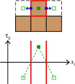 図4. 速度の水平成分が必ず0になってしまう格子セル(赤枠)。 Fig. 4. Grid cells (shown by the red frame) where the horizontal velocity is necessarily zero. |